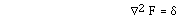
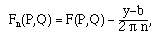
![Integral G(P,Q) f(P) dpA = Integral G(P,Q) --p<sup>2</sup>u(P)
dpA
= Integral --p.[G(P,Q) --pu - --pG(P,Q) u] dpA + Integral
--p<sup>2</sup>G(P,Q) u(P) dpA
= - Integral [[partialdiff]]G/[[partialdiff]][[eta]](P,Q) u(P) dps +
Integral d(P,Q) u(P) dpA
= - Integral [[partialdiff]]G/[[partialdiff]][[eta]](P,Q) g(P) dps +
Integral d(P,Q) u(P) dpA.](pix/jvhgIII6a1.GIF)
Linear Methods of Applied Mathematics
Evans M. Harrell II and James V. Herod*
In this section we shall construct Green functions for the problems of the type: Find u such that
grad2u = f on D,
u = g on the boundary of D.
(17.1)
In order to simplify notation, we will let P or Q represent points in the plane. For example, P might represent {x,y} and Q represent {a,b}. We indicate that in two dimensions,
grad2G(P,Q) = Gxx + Gyy,
instead of partials with respect to a and b, by writing gradp2G(P,Q).
The function G is to be constructed to have these properties:
gradp p2 G(P,Q) = \delta(P,Q)
and
G(.,Q) = 0 on the boundary of D
(17.2)
(Dirichlet type boundary conditions). Having such a G, the following applications of Green's identities show that we can determine the solution to the partial differential equation:
Thus, having such a G and knowing f and g, we have a formula for u which provides a solution to the problem:
![u(Q) = Integral G(P,Q) f(P) dpA + Integral
[[partialdiff]]G/[[partialdiff]][[eta]](P,Q) g(P) dps.](pix/jvhgIII6a2.GIF)
How is such a G constructed? We will do it in two pieces. We construct G = F + R where F is the free Green function (also known as the fundamental or singular part) and satisfies
 on all of R2
and
on all of R2
and
F (.,Q) is independent of \theta (in polar coordinates).
(17.3)
R is the regular part and satisfies
![grad<sup>2</sup> R = 0 on D, R = - F on [[partialdiff]]D.](pix/jvhgIII6a4.GIF)
(17.4)
Let us recall that whenever we have a linear, inhomogeneous problem, the general solution is given by any particular solution, plus the general solution of the related homogeneous problem. Equation (17.4) is the homogeneous equation associated with (17.3). It has no delta function, so its solutions will be completely regular. (Even if the boundary conditions were rough this is guaranteed by a general theorem for Laplace's equation.)
In other words, the singular parts of any two Green functions for the same equation, but different boundary conditions, will be the same. So let us find that singular part in the simplest possible situation, which is (17.3).
FINDING THE FREE GREEN FUNCTION
We begin by constructing F. Recall the formula for --2 in polar coordinates:
![grad<sup>2</sup>u = F(1,r)
F([[partialdiff]](r[[partialdiff]]u/[[partialdiff]]r) ,[[partialdiff]]r) +
F(1,r<sup>2</sup>)
F([[partialdiff]]<sup>2</sup>u,[[partialdiff]][[Theta]]<sup>2 ) </sup>.](pix/jvhgIII6a5.GIF) (17.5)
(17.5)
In seeking F such that
, we recall that, in the sense of
distributions, \delta({x,y},{a,b}) = 0 unless {x,y} = {a,b}. Also, \delta is radially
symmetric. Thus, supposing initially that Q = {a,b} is at the origin, we have
![0 = grad<sup>2</sup>F = 1/r
[[partialdiff]](r[[partialdiff]]F/[[partialdiff]]r)/[[partialdiff]]r +
1/r<sup>2</sup>
[[partialdiff]]<sup>2</sup>F/[[partialdiff]][[Theta]]<sup>2</sup> <sup></sup><p>
<sup></sup> = 1/r [[partialdiff]](r
[[partialdiff]]F/[[partialdiff]]r)/[[partialdiff]]r.](pix/jvhgIII6a6.GIF)
This last equality is because F is independent of \theta. Thus r Fr is constant and F(r) = A ln(r) + B for some A and B. It remains to find A and B. To this point we have not used information about F at the origin, only at {x,y} different from {0,0}. Information about F at {a,b} comes through the integral. If we integrate the delta function over any disk with radius c > 0 we get 1, so:
![1 = Integral --<sup>2</sup>F dA = Integral --.-- F dA = Integral; gradF.[[eta]] ds](pix/jvhgIII6a7.GIF)
by the divergence theorem. Since F is radially symmetric, we can calculate the last integral as
Thus, A = 1/(2 \pi) and B is undetermined. We may as well choose it to be 0 at this stage. Of course there is no singularity in the constant function, so its derivatives do not contribute to the delta function. When Q is not at the origin, we simply shift the calculation by Q:
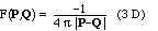
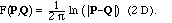
F(P,Q) = ln[|P - Q|]/(2 \pi).
In coordinates
F({x,y},{a,b}) = ln[ (x-a)2 + (y-b)2]/(4 \pi)
(the factor of 1/2 comes because ln(ra) = a ln(r)).
The function F is the Green function for the following problem:
This problem is in the first alternative, as a consequence of a theorem of Liouville for solutions of Laplace's equation (known as harmonic functions ), which implies that the only square-integrable solution is 0. See exercise 3 for why the assumption that u is square integrable is necessary. Some mild assumptions on f are needed, for instance |f| could be assumed bounded by any large constant times (1 + r)-3.
THE METHOD OF IMAGES
Model Problem III.6a. Now let us solve the problem (17.1) on a new domain, the upper half plane, where x may have any value but y > 0. We need to find a Green function which = 0 when y = 0.
Solution. We may as well imagine that the problem we wish to solve is (17.1) for y > 0, with the boundary condition
u(x,0) = 0,
for it has the same Green function as other with more complicated Dirichlet boundary data on the x-axis, as shown above.
Here are two ways to derive the Green function.
I. Because (17.1) is a well-posed problem, it has a unique solution. Thus if we can find a solution by imagining a different situation which is easier to solve, but which satisfies the partial differential equation and the boundary condition, it must be the right solution. The different situation will be one on all of R2, like the problem we just solved, but where the boundary condition happens to be satisfied. Here is how:
Since f(x,y) is physically meaningful only for y > 0, we are free to define it however we will when y < 0. Let us choose to define it by the odd extension , so f(x,-y) = - f(x,y). We can solve this modified problem with the free Green function, as
(17.6)
The last step here came from rewriting the integral over y < 0 using the odd symmetry. Notice that if y=0, this integral vanishes, while for y > 0, the extended function f has the same values as posited in the problem. Because of uniqueness, it is the right solution to the problem on the upper half plane. The Green function for the half-plane problem is
G(P,Q) = F(P,Q) - F(PR,Q),
(17.7)
where PR = {x,-y} is the point found by reflecting P across the x-axis. It is as if there were an equal and opposite image source for the problem, located in the lower half plane.
II. Here is another way to derive the solution (17.6) and the Green function (17.7). As remarked above, the Green function for this problem is of the form
G(P,Q) = F(P,Q) + R(P,Q),
where R is a regular function, solving Laplace's equation on the domain D where the problem resides, in this case the upper half plane. Can we find such a solution, such that G will satisfy a zero Dirichlet boundary condition? Yes, because the function F(S,Q) solves
--2 F(S,Q) = 0
(in the Q variable) for any S which is not in the domain D, since the delta function is zero everywhere except at the singularity. Taking S = PR and R(P,Q) = - F(PR,Q) gives a Green function which is 0 when y=0, as required.
Let's use the method of images to solve some more problems.
Model Problem III.6b. We continue to solve Poisson's equation (17.1), but now on the strip D = {x unrestricted, 0 < y < 1}. Dirichlet boundary conditions are imposed on the strip.
Solution. Have you ever been in a barber shop or hair dresser where you sit between two mirrors? You see an infinite number of reflections of yourself, alternating as to whether they face toward you or away from you. If we want to place image Green functions in the plane to match both boundary conditions, we need an infinite number of them. The position reflected from height y<1 through y=1 is 2 - y (when y=0 the reflection is at 2 and when y=1 it meets its reflection). The next reflection will be at 2+y, the next one at 4 - y, and so forth. We need to alternate signs to get all the cancellations. The result ought to be:

There is a subtlety here, however, which is that the infinite sums do not converge separately; this expression is off the form
infinity - infinity.
Remember, however, that we can subtract a regular solution of Laplace's equation

to the free Green function, so long as we end up satisfying the boundary condition. There is more than one way to do this, but the simplest one to use here (see exercise) is
(17.8)
and to sum the images in the following way:

(17.9)
(It should be easy to see that c (y-b) solves Laplace's equation for any b,c.)
Model Problem III.6c. We continue to solve Poisson's equation (17.1), again on the upper half-plane y>0, but this time with Neumann-type boundary conditions,
uy(x,0) = 0.
Solution. The Green function we need this time uses the even reflection through y=0. The Green function with the correct boundary condition is:
G(P,Q) = F(P,Q) + F(PR,Q).
(17.10)
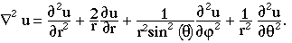
In some ways things are simpler in three dimensions for this problem. Let us now seek the three-dimensional free Green function with the same technique as we used above. We begin by looking for a solution of Laplace's equation which depends only on the radial coordinate in the spherical coordinate system. In this system, the Laplace operator has the form
So if the point Q is put at the origin, the free Green function will satisfy the ordinary differential equation
F'' + 2 F'/r = 0
in r for all r > 0. The solutions of this are of the form F = A/r + B.
Again, we may choose B = 0 in most circumstances, and use the divergence theorem to evaluate A:
1 = Integral --2F dV = Integral --.-- F dV = Integral -- F.[[eta]] dA
(see above). Since F is radially symmetric, we can calculate the last integral as
= - Integral A/r2 dA = -4 pi A.
We conclude that in three dimensions,
F(P,Q) = - 1/(4 pi |P - Q|).
For those of you who have an interest in electromagnetism, this may be familiar as the electric potential of a unit charge (with a certain choice of physical units and a sign convention which may be the opposite of what you will find in a physics class). If there is a continuous charge distribution f(P), then the electrostatic potential in free space is the solution of
--2u = f
i.e.,
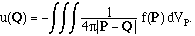
You can think of this as a continuous superposition of the potentials due to point charges, distributed according to the function f.
The method of images works in three dimensions just as in two dimensions:
Model Problem III.6d. Now let us solve Poisson's equation on the upper half space, where x and y may have any value but z > 0. We need to find a Green function which = 0 when z = 0.
Solution: If P = {a,b,c} and Q = {x,y,z}, then the Green function is:

G(P,Q) := F(P,Q) - q F(P,Q'),
where the "charge" q > 1, then G will be negative for P sufficiently near Q and positive for P sufficiently near Q', since the Free Green function diverges to - infinity at its singularity. The function G must also be positive very far away from Q and Q', for the assumption that q > 1 means that the second contribution is more important at large distances: Physically speaking, a probe at a large distance will detect the net charge, q-1. (In physics the sign convention is that a positive point charge corresponds to the Green function -F, so the sign is reversed from what you might guess.) Clearly, G = 0 on some region surrounding Q but not Q'.
In order to determine this region, let us choose the x-axis so that
Q = {a1, 0, 0} and Q' = {a2, 0, 0}.
The region must be rotationally symmetric about the x-axis, so to determine it we can set z = 0. The coordinates of the points in the y-z plane where G = 0 thus satisfy
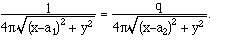
This is equivalent to
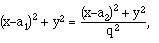
when we take reciprocals of both sides and square. Collecting terms, we get
This is the equation of a circle with a center somewhere on the x-axis! If we do not specialize to the x-y plane and points Q and Q' on the x-axis, we must conclude:
F(P,Q) - q F(P,Q') = 0
precisely on some sphere when q > 1.
Armed with this knowledge, it is a matter of algebra to go the other way and find the values of Q' and q which produce the correct Green function for any particular sphere. Supposing that the sphere is centered at the origin and has radius R. If Q = (a1,0,0) we find:
a2 = R2/a1
q = -R/a1.
(17.11)
If Q is not located on the x-axis, we can find q and Q' simply by rotating this relationship: Q' = Q R2/|Q|2, and q = R/|Q|.
Theorem. The Green function for Poisson's equation in the sphere of radius R (or, in two-dimensions, the circle of radius R), with Dirichlet boundary conditions, is
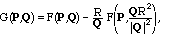
where F is the free Green function
or
XVII.1. Derive the formula for the Laplacian in polar coordinates (17.5) by making a change of variables.
XVII.2. Derive the formula for the Laplacian in parabolic coordinates by making a change of variables to
u = (x2+y2)1/2 + x,
v = (x2+y2)1/2 - x,
XVII.3. Show that all of the following are harmonic functions (solutions of Laplace's equation), but that they are not square integrable:
a) c (y - b), for any constants b and c
b) x + 3 y
c) x y + 1
d) x2 - y2
e) cos(x) sinh(y)
XVII.4. Do the explicit calculation to show that if G is defined by (17.9), then
Gy({x,y}, Q) = 0 when y = 0.
XVII.5. Use a Taylor expansion (in 1/n) to show that the terms in the series (17.9), with Fn defined by (17.8), are bounded by C/n2 for some constant C (independent of x and y), and that the series thus converges.
XVII.6. Solve Poisson's problem in the first quadrant in two dimensions with boundary conditions:
u(x,0) = 0;
ux(0,y) = 0.
XVII.7. Solve Poisson's problem in two dimensions with Neumann boundary conditions on the strip 0 < y < 1:
uy(x,0) = uy(x,1) = 0
Hint. The corrected Green function in (17.8) will not be good enough for convergence this time. A better, but more complicated correction will be
F({x,y+2n},{a,b}) - (y-b)/(2 \pi n) - ln(2) /(2 \pi) - ln(n)/(2 \pi).
XVII.8. Solve the problem
where r is the radial coordinate, on the full three-dimensional space R3.
XVII.9. Solve the problem
where f(x) = 1 for |x| < 2 and 0 otherwise, on the domain x < 4, y and z unrestricted. Impose the boundary condition.
u(4,x,,y) = 0
XVII.10. Find the ordinary differential equation for the free Green function for the Helmholtz equation in two dimensions,
where k is a nonzero constant.
(The solutions of this equation are known as modified Bessel functions.)
XVII.11. Solve Poisson's equation in the sphere of radius 1 with charge distribution f(Q) = 1 for 1/2 < |Q| < 1, and 0 otherwise. XVII.12. Find the Green function for Poisson's equation a) within the hemisphere x2 + y2 + z2 = 1, z > 0, with zero Dirichlet